Minimal MVLEM Example

Original Post - 07 Jul 2024 - Michael H. Scott

Visit Structural Analysis Is Simple on Substack.

Due to its simplicity and efficiency in modeling shear walls, the MVLEM (Multiple Vertical Line Element Model) is among the more frequently asked about elements in OpenSees. The MVLEM is also one of the better documented elements in OpenSees with documentation for both its 2D and 3D versions.

Personally, I haven’t used the MVLEM for anything more than basic tests–like a single element model for checking sendSelf and recvSelf. And the extent of my shear wall knowledge is an example that I use in an undergraduate class in Eastchester.

Three story wall model

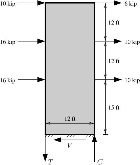
Despite my limited wall modeling experience, I know that using MVLEM elements should give the expected base shear and chord forces, V=68 kip and T=C=143 kip, respectively, for this statically determinate wall. Also, the model I will show is elastic, so let’s not get hung up on the magnitude of the loads. Maybe a small earthquake or perhaps a stiff breeze. Whatever.

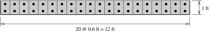
Let’s say the wall is 1 ft thick and the materials are all elastic with concrete modulus E_c=3600 ksi and Poisson ratio v=0.25, and steel modulus E_s=29000 ksi. The wall section consists of 20 vertical line elements, a.k.a., “fibers”, of equal size. Although more longitudinal steel would be placed in the chords than in the field, for simplicity, I’ll use 1% steel reinforcing ratio in each concrete line element. Like the load magnitudes, let’s not get hung up on the reinforcing details either.

Wall cross-section

Whether you use the MVLEM in 2D or 3D models, you have to define the wall section properties in lists. You can adjust the fiber sizes and reinforcing ratios after getting comfortable with the results of this simple analysis.

import openseespy.opensees as ops

kip = 1
inch = 1
ft = 12*inch

ksi = kip/inch**2

b = 1*ft
h = 12*ft

Ec = 3600*ksi
v = 0.25
Gc = 0.5*Ec/(1+v)
Es = 29000*ksi

N = 20
rho = 0.01

ops.uniaxialMaterial('Elastic',1,Ec)
ops.uniaxialMaterial('Elastic',2,Es)

conc = [1]*N
steel = [2]*N
rhoList = [rho]*N
bList = [b]*N
hList = [h/N]*N

In addition, just like what one would do with a section aggregator, the shear force-deformation response of each wall element is described by its own uniaxial material, separate from the fiber-based flexural response.

A = b*h
ops.uniaxialMaterial('Elastic',3,Gc*A)
shear = 3

The above material definitions will be used for the following 2D and 3D analyses of the wall.

Two-Dimensional Model

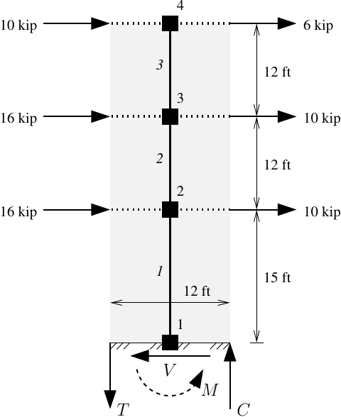
The two-dimensional version of MVLEM is a two node element. Accordingly, four nodes are defined along the centerline of the wall model.

Wall model with 2D MVLEM elements

The model is defined below with the following notes:

For some unknown reason, the element density, which is rarely used, even in dynamic analysis, is the first required argument after the element tag. Thus, the 0.0 before the node tags.
The center of rotation of each MVLEM element, measured from end I, is specified as 0.4 times the element height, the recommended value.

ops.wipe()
ops.model('basic','-ndm',2,'-ndf',3)

ops.node(1,0,0); ops.fix(1,1,1,1)
ops.node(2,0,15*ft)
ops.node(3,0,27*ft)
ops.node(4,0,39*ft)

#
# Materials and fiber lists defined above
#

ops.element('MVLEM',1,0.0,1,2,N,0.4,'-thick',*bList,'-width',*hList,'-rho',*rhoList,'-matConcrete',*conc,'-matSteel',*steel,'-matShear',shear)
ops.element('MVLEM',2,0.0,2,3,N,0.4,'-thick',*bList,'-width',*hList,'-rho',*rhoList,'-matConcrete',*conc,'-matSteel',*steel,'-matShear',shear)
ops.element('MVLEM',3,0.0,3,4,N,0.4,'-thick',*bList,'-width',*hList,'-rho',*rhoList,'-matConcrete',*conc,'-matSteel',*steel,'-matShear',shear)

ops.timeSeries('Linear',1)
ops.pattern('Plain',1,1)

ops.load(2,26*kip,0,0)
ops.load(3,26*kip,0,0)
ops.load(4,16*kip,0,0)

ops.analysis('Static','-noWarnings')
ops.analyze(1)

ops.reactions()

V = ops.nodeReaction(1,1) # base shear
C = ops.nodeReaction(1,3)/h # base chord force

Note that the chord force is found by dividing the moment reaction at the base of the wall by the wall width. Printing the reactions, you should get V=68 kip and T=C=143 kip, with some slight round off. Also, the lateral displacement at the top of the wall is 0.116 inch.

Three-Dimensional Model

The MVLEM for three-dimensional models is a four node element. As a result, we need eight nodes for this wall model–two nodes at the base and two nodes at each floor.

Wall model with 3D MVLEM elements

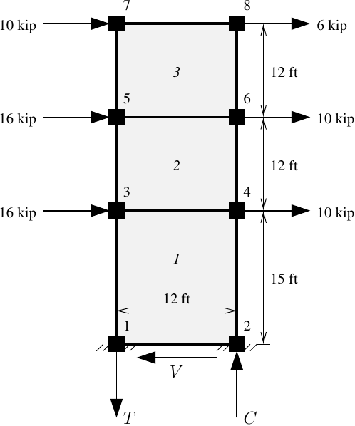
The 3D MVLEM uses the same formulation for in-plane response as the 2D version. Rigid constraints (stiff imaginary beams) are used within the 3D element to transform displacements from the four nodes down to the centerline.

In addition, note the following for the 3D MVLEM:

The element density is not required for the 3D MVLEM. Thus, no 0.0 betwixt the element and node tags.
The center of rotation, measured perpendicular from the I-J edge of the element, is the recommended value of 0.4 times the element height.
Whether the base nodes are pinned (as shown below) or fixed does not matter much for the MVLEM, at least not for this analysis.
The 3D MVLEM Frankensteins linear-elastic plate equations for the out-of-plane response. The plate stiffness is determined from the section geometry and the initial stiffness of the uniaxial materials assigned to the concrete fibers and a user specified Poisson ratio (default=0.25). For nonlinear in-plane response, the assumption of elastic out-of-plane response deserves some scrutiny.

ops.wipe()
ops.model('basic','-ndm',3,'-ndf',6)

ops.node(1,0,0,0); ops.fix(1,1,1,1,0,0,0)
ops.node(2,h,0,0); ops.fix(2,1,1,1,0,0,0)
ops.node(3,0,0,15*ft)
ops.node(4,h,0,15*ft)
ops.node(5,0,0,27*ft)
ops.node(6,h,0,27*ft)
ops.node(7,0,0,39*ft)
ops.node(8,h,0,39*ft)

#
# Materials and fiber lists defined above
#

ops.element('MVLEM',1,1,2,4,3,N,0.4,'-thick',*bList,'-width',*hList,'-rho',*rhoList,'-matConcrete',*conc,'-matSteel',*steel,'-matShear',shear)
ops.element('MVLEM',2,3,4,6,5,N,0.4,'-thick',*bList,'-width',*hList,'-rho',*rhoList,'-matConcrete',*conc,'-matSteel',*steel,'-matShear',shear)
ops.element('MVLEM',3,5,6,8,7,N,0.4,'-thick',*bList,'-width',*hList,'-rho',*rhoList,'-matConcrete',*conc,'-matSteel',*steel,'-matShear',shear)

ops.timeSeries('Linear',1)
ops.pattern('Plain',1,1)

ops.load(3,16*kip,0,0,0,0,0)
ops.load(4,10*kip,0,0,0,0,0)
ops.load(5,16*kip,0,0,0,0,0)
ops.load(6,10*kip,0,0,0,0,0)
ops.load(7,10*kip,0,0,0,0,0)
ops.load(8, 6*kip,0,0,0,0,0)

ops.analysis('Static','-noWarnings')
ops.analyze(1)

ops.reactions()

V = ops.nodeReaction(1,1) + ops.nodeReaction(2,1) # base shear
C = ops.nodeReaction(2,3) # base chord force

Print the reactions. Like the 2D model, you should get V=68 kip and T=C=143 kip with some round off discrepancies. And the lateral displacement at the top of the wall is 0.116 inch, matching the 2D analysis.

Summary

The MVLEM is pretty straightforward–basically a beam element with a single fiber section and an aggregated shear force-deformation relationship. After you get comfortable with this example, start making minor tweaks like changing the concrete material from Elastic to ENT (elastic-no-tension), then keep doing more analyses.

The SFI_MVLEM and E_SFI_MVLEM (SFI stands for Shear-Flexure Interaction), which use multi-axial material models (nDMaterial) to couple axial and shear stresses in each fiber, will be discussed in a separate post.

OpenSees Cloud

OpenSees AMI

Minimal MVLEM Example

Two-Dimensional Model

Three-Dimensional Model

Summary