OpenSees Cloud

OpenSees AMI

Monte Carlo Simulation with OpenSeesMP

Original Post - 20 Jul 2024 - Michael H. Scott

Visit Structural Analysis Is Simple on Substack.

The parallel computing capabilities of OpenSeesSP and OpenSeesMP are easily confused.

OpenSeesSP runs your script on a single processor with the other processors awaiting instructions on what to do. OpenSeesSP is ideal for assigning subdomains of a large model to each processor. The main processor, processor 0, directs traffic and solves the governing equations of equilibrium along the domain partitions.

A lot of magic happens behind the scenes of an OpenSeesSP analysis, most of which is out of your control–like whether or not I correctly implemented sendSelf and recvSelf for Concrete23 and CadillacBeamColumn.

On the other hand, you are in the driver’s seat with OpenSeesMP.

OpenSeesMP runs a copy of your script on every processor and is thus suited for embarrassingly parallel tasks like Monte Carlo simulation or analyses for a large suite of ground motions or load cases. Minimal logic is required to make sure each processor analyzes something different, e.g., for a unique set of parameter values or for distinct ground motions.

A handful of commands are available in the parallel interpreters (Tcl and Python) to facilitate OpenSeesMP analyses.

• getNP() - returns the number of processors, N, available for this analysis
• getPID() - returns the ID for this processor, from 0 to N-1
• send('-pid',pid,data) - sends data from this processor to the processor with ID pid; although data can be a double, it’s usually best to send a string of information that the recipient processor can split and cast
• recv('-pid',pid) - the return value for this function is the data (double or string) sent by the processor with ID pid
• barrier() - inserts a point in your script that all processors must reach before script execution continues

Note that the send and recv commands have nothing to do with the sendSelf and recvSelf methods I complained about earlier in this post, and in other posts.

Any way, let’s see how to use the OpenSeesMP commands for Monte Carlo simulation of the toy reliability problem from ADK’s Structural and System Reliability.

The script below creates two Nataf-distributed random variables and counts how many realizations lead to a failure state for the toy limit state function, $g = X_1^2 - 2X_2$. Each realization of random variables is based on random values from the standard normal distribution transformed to the standard space.

import openseespy.opensees as ops
import random

Ntrials = 1000000 # Total number of trials

Nproc = ops.getNP()
NtrialsProc = Ntrials // Nproc # integer division
Ntrials = NtrialsProc * Nproc 

ops.randomVariable(1,'lognormal','-mean',10.0,'-stdv',2.0)
ops.randomVariable(2,'gumbel','-mean',20.0,'-stdv',5.0)

ops.correlate(1,2,0.5)

ops.probabilityTransformation('Nataf')

# Limit state function
def g(X):
    return X[0]**2 - 2*X[1]

nrv = len(ops.getRVTags())

Nfail = 0
for i in range(NtrialsProc):
    U = [random.gauss(0,1) for _ in range(nrv)]
    X = ops.transformUtoX(*U)
    if g(X) < 0:
        Nfail += 1

pid = ops.getPID()
print(f'Processor {pid}, Nfail = {Nfail}',flush=True)

ops.barrier()

if pid == 0:
    for i in range(1,Nproc):
        data = ops.recv('-pid',i)
        data = data.split()
        Nfail += int(data[0])
    print('Total pf:',Nfail/Ntrials)
else:
    ops.send('-pid',0,f'{Nfail}')

The trials are distributed to N processors, then each processor sends its results to processor 0, who tallies the trials and computes the probability of failure. (Any processor can do the sums, but the scripting is cleaner when processor 0 collects results). The barrier ensures processor 0 doesn’t do the sums and move on before other processors have a chance to finish.

Running the script with mpiexec on four processors gives the following output.

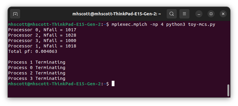
The estimated probability of failure, 0.406%, is similar to the FORM approximation of 0.362%.

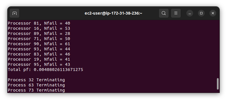
Using 96 processors on a c5.metal instance of the OpenSees virtual machine, gives similar results with each processor doing fewer trials.

Yeah, 96 processors is overkill for Monte Carlo simulation of the toy reliability problem and you won’t see significant speed up because each trial is so simple. But this post showed the basic framework for performing Monte Carlo Simulation with OpenSeesMP and you can swap out the toy limit state function for finite element models.