OpenSees Cloud
OpenSees AMI
A Return to FORM
10 Nov 2024 - Michael H. Scott
The structural reliability modules Terje Haukaas implemented in OpenSees comprised one of the last groups of commands to be ported from Tcl to Python. So, performing reliability analysis in OpenSeesPy has been slow to catch on. But the porting is done and there are some slight differences between Tcl and Python.
This post shows basic FORM (first order reliability method) analyses using OpenSeesPy. The structural model is a simple truss.
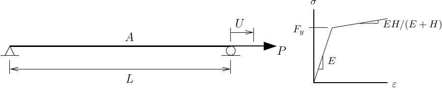
The model and reference load are defined below.
import openseespy.opensees as ops

# Units = kip,inch
E = 29000
Fy = 50
Hkin = 500

A = 10
L = 100

ops.wipe()
ops.model('basic','-ndm',2,'-ndf',2)

ops.node(1,0,0); ops.fix(1,1,1)
ops.node(2,L,0); ops.fix(2,0,1)

ops.uniaxialMaterial('Hardening',1,E,Fy,0,Hkin)

ops.element('truss',1,1,2,A,1)

ops.timeSeries('Linear',1)
ops.pattern('Plain',1,1)
ops.load(2,1.0,0)
The deterministic response (using the given values of the model parameters) up to a load of 600 kip is shown below. At the peak load, the displacement is about 2.2 inch.
PLOT
After defining the model, we can define random variables then map those
random variables to objects in the model. The material properties are
assigned lognormal distributions while the cross-sectional area of the
truss is assigned a normal distribution. Each random variable takes a
tag, mean, and standard deviation. The random variables are
uncorrelated. Detailed joint PDFs are not point of this post.
ops.randomVariable( 9,'lognormal','-mean',E,'-stdv',0.02*E)
ops.randomVariable(16,'normal','-mean',A,'-stdv',0.05*A)
ops.randomVariable(25,'lognormal','-mean',Fy,'-stdv',0.15*Fy)
ops.randomVariable(36,'lognormal','-mean',Hkin,'-stdv',0.2*Hkin)

ops.probabilityTransformation('Nataf')
Even though the random variables are uncorrelated, we’ll use the Nataf
transformation between original and standard normal spaces. Nataf will
always work in place of AllIndependent for uncorrelated random
variables, just like Newton will always work in lieu of Linear for the
equilibrium solution of linear models.
We can then map parameters to the random variables. The tags of the parameters don’t really matter. The arguments after the random variable tag drill down to the setParameter methods of the element and its material.
ops.parameter(1,'randomVariable', 9,'element',1,'E')
ops.parameter(3,'randomVariable',16,'element',1,'A')
ops.parameter(5,'randomVariable',25,'element',1,'Fy')
ops.parameter(8,'randomVariable',36,'element',1,'Hkin')
Regardless of the analysis (we’ll do a load control and a displacement
control analysis of the truss), some of the reliability options will be
the same. We will start the search for the design point at the mean
values of all the random variables, use the improved HLRF algorithm with
a fixed step size to search for the design point, and set absolute and
relative convergence tolerances of 1e-2 on the performance function
being close to zero.
ops.startPoint('Mean')
ops.searchDirection('iHLRF')
ops.stepSizeRule('Fixed','-stepSize',1.0)
ops.reliabilityConvergenceCheck('Standard','-e1',1e-2,'-e2', 1e-2,'-print',1)
All of these options are pretty standard; however, you may want to use
the Armijo step size rule for more complex reliability analyses.
Load Control Analysis
In a load control analysis, we’re interested in the displacement not exceeding a specified threshold. For the sake of demonstration, let’s use a displacement limit of 3.5 inch. The performance function is then g = 3.5 - U, such that when g is less than zero, the system does not satisfy the performance objective.
Py = A*Fy
Pmax = 1.2*Py

Nsteps = 100
dP = Pmax/Nsteps
ops.integrator('LoadControl',dP)

ops.performanceFunction(1,'3.5-ops.nodeDisp(2,1)')
In addition to the performance function, we need the gradient of the performance function with respect to each random variable. In this case, the gradient of the performance function is easy, \(\partial g/\partial X_j = -\partial U/\partial X_j\); however, defining these gradients for each random variable would be cumbersome.
Fortunately, there are helper functions: getRVTags returns a list of
currently defined random variables and getRVParamTag returns the
parameter tag to which a given random variable is mapped. With these two
functions, we can define the simple expressions for the gradient of the
performance function with respect to each parameter.
for rv in ops.getRVTags():
    param = ops.getRVParamTag(rv)
    ops.gradPerformanceFunction(1,rv,f'-ops.sensNodeDisp(2,1,{param})')
Now, we can define how to evaluate the performance function and how and when to evaluate the gradients of the performance function.
For monotonic loading, we only need to evaluate gradients
(sensitivities) at the end of the analysis. In this case, we can use the
-computeByCommand option for the sensitivity algorithm. Then put two
commands in the functionEvaluator: analyze and compute gradients.
ops.sensitivityAlgorithm('-computeByCommand')
ops.functionEvaluator('Python','-file',f'ops.analyze({Nsteps}); ops.computeGradients()')
Alternatively, we can compute gradients at each (pseudo-)time step, in
which case we don’t need to tell the functionEvaluator to compute
gradients, i.e., the gradients are computed automatically.
ops.sensitivityAlgorithm('-computeAtEachStep')
ops.functionEvaluator('Python','-file',f'ops.analyze({Nsteps})')
For large models with many random variables, you don’t want to compute the gradients at every time step if you don’t have to do so.
After the functionEvaluator is defined, we indicate how to evaluate the
gradient of the performance function: either implicitly via the
DDM (direct differentiation method)
or by
finite differences.
ops.gradientEvaluator('Implicit') # DDM
#ops.gradientEvaluator('FiniteDifference')
The DDM is not available for all element and material models in OpenSees. Finite differences should work for any element or material for which the setParameter and updateParameter methods are implemented. But finite differences can be very slow for large models with many random variables.
Finally, to run the FORM analysis, we declare the algorithm to find the
design point, then issue the runFORMAnalysis command with an output
filename.
ops.findDesignPoint('StepSearch','-maxNumIter', 15)

ops.runFORMAnalysis('truss-load-control-FORM.out')
After running the analysis, the output file should have the following contents.
#######################################################################
#  FORM ANALYSIS RESULTS, LIMIT-STATE FUNCTION NUMBER 1               #
#                                                                     #
#  Limit-state function value at start point: ......... 1.2931        #
#  Limit-state function value at end point: ........... 0.00121       #
#  Number of steps: ................................... 2             #
#  Number of g-function evaluations: .................. 15            #
#  Reliability index beta: ............................ 0.67121       #
#  FO approx. probability of failure, pf1: ............ 2.51043e-01   #
#                                                                     #
# rvtag   x*          u*         alpha    gamma    delta    eta       #
#  9    2.899e+04  -1.661e-03  -0.00242 -0.00242     -        -       #
#  16   9.869e+00  -2.611e-01  -0.38812 -0.38812     -        -       #
#  25   4.547e+01  -5.614e-01  -0.84130 -0.84130     -        -       #
#  36   4.658e+02  -2.593e-01  -0.37627 -0.37627     -        -       #
#                                                                     #
#######################################################################
The output file includes the reliability index, design point realizations of the random variables, and the importance measures, along with other information. The load-displacement response of the truss is shown below for the mean values of the random variables and the realizations at the design point.

Displacement Control Analysis
Instead of a load control analysis to determine the probability of exceeding a displacement threshold, we can perform a displacement control analysis to determine the probability that the load carrying capacity of the truss will be less than 500 kip at the mean value of displacement of about 2.2 inch.
In this case, the limit state function is g = P - 500 and the gradient of the performance function is \(\partial g/\partial X_j = \partial P/\partial X_j\).
Umax = 2.2
Nsteps = 100
dU = Umax/Nsteps
ops.integrator('DisplacementControl',2,1,dU)

ops.performanceFunction(2,`ops.getLoadFactor(1)-500`)
for rv in ops.getRVTags():
    param = ops.getRVParamTag(rv)
    ops.gradPerformanceFunction(2,rv,f'ops.sensLambda(1,{param})')
Because the reference load is 1.0, the load factor is the applied load, P.
Everything else from the FORM analysis with load control will be the same, we just send the reliability analysis results to a different file.
ops.runFORMAnalysis('truss-displacement-control-FORM.out')
The output file is shown below.
#######################################################################
#  FORM ANALYSIS RESULTS, LIMIT-STATE FUNCTION NUMBER 2               #
#                                                                     #
#  Limit-state function value at start point: ......... 99.661        #
#  Limit-state function value at end point: ........... 0.06073       #
#  Number of steps: ................................... 2             #
#  Number of g-function evaluations: .................. 15            #
#  Reliability index beta: ............................ 1.2476        #
#  FO approx. probability of failure, pf1: ............ 1.06088e-01   #
#                                                                     #
# rvtag   x*          u*         alpha    gamma    delta    eta       #
#  9    2.899e+04  -2.910e-03  -0.00231 -0.00231     -        -       #
#  16   9.765e+00  -4.708e-01  -0.37835 -0.37835     -        -       #
#  25   4.191e+01  -1.109e+00  -0.88792 -0.88792     -        -       #
#  36   4.597e+02  -3.254e-01  -0.26162 -0.26162     -        -       #
#                                                                     #
#######################################################################
And below is the truss load-displacement response for the mean values of the random variables and the realizations at the design point.
