Hydrostatic Loading on a Wall

Original Post - 13 Nov 2024 - Michael H. Scott

Visit Structural Analysis Is Simple on Substack.

One of the simplest examples of fluid-structure interaction is hydrostatic loading on a beam, an analysis the PFEM in OpenSees should be able to handle.

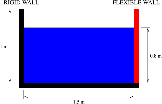
Suppose the right wall of the tank shown below is a 1.25 cm (1/2 inch) thick steel plate, which we can model with beam elements in two dimensions. The left wall and the bottom of the tank are fixed and rigid.

This example is similar to an example from Zhu and Scott (2016). Probably done in Tcl, so here’s the highlights for Python.

To accommodate beam elements in the tank definition, we use 3 DOF/node. We define a mesh of nodes for the left wall and tank floor, then fix all DOFs. For the right wall, we define a mesh of beam elements using the material properties and dimensions of the plate.

import openseespy.opensees as ops

ops.wipe()
ops.model('basic','-ndm',2,'-ndf',3)

kg = 1
m = 1
sec = 1

N = kg*m/sec**2
Pa = N/m**2

g = 9.81*m/sec**2

# Tank dimensions
Ltank = 1.5*m
Htank = 1*m
hfluid = 0.8*m
tfluid = 0.5*m

ops.node(1,0,Htank)
ops.node(2,0,0)
ops.node(3,Ltank,0)
ops.node(4,Ltank,Htank)

meshsize = 0.02*m

# Create tank walls and floor
sid = 1
walltag = 1
ops.mesh('line',walltag,3,*[1,2,3],sid,3,meshsize)

wallnodes = ops.getNodeTags('-mesh', walltag)
for nd in wallnodes:
    ops.fix(nd, 1, 1, 1)

# Plate dimensions
b = tfluid
tp = 0.0125*m # 1.25 cm
E = 200e9*Pa
rhos = 7850*kg/m**3

beamtag = 2
ops.geomTransf('Corotational',1)
A = b*tp
I = b*tp**3/12
ops.mesh('line',beamtag,2,3,4,sid,3,meshsize,'elasticBeamColumn',A,E,I,1,'-mass',rhos*A)

beamnodes = ops.getNodeTags('-mesh', beamtag)

For this model and analysis, the corotational transformation is unnecessary, but would be appropriate for modeling more flexible frame structures that undergo large displacements under fluid loading.

Anyway, the definition of the background mesh and fluid elements is the same as in the hydrostatic analysis shown in this post.

The analysis uses time steps of 0.005 sec out to a final time of 1.5 sec, which should be long enough for the steel plate to reach static equilibrium, more or less. At each time step, we assemble the reactions for subsequent plotting (with the -dynamic option to include element inertia) and re-mesh the fluid domain.

ops.analysis('PFEM', 5e-3*sec, 5e-3*sec, -g)

totaltime = 1.5*sec

while ops.getTime() < totaltime:

    # Analyze at current time step
    if ops.analyze() < 0:
        break

    ops.reactions('-dynamic')

    ops.remesh()

Using the statically determinate idealization shown below, we know exact solutions based on strength of materials and hydrostatic fluid loading on a beam.

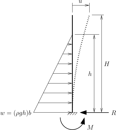
The horizontal reaction at the base of the wall is R=wh/2, where \(w=(\rho gh)b\) is the peak intensity of the hydrostatic pressure multiplied by the tributary width. The moment reaction at the base is M=wh²/6 and the exact static solution for the deflection at the top of the wall is u=wh⁴/(30EI)+(H-h)wh³/(24EI).

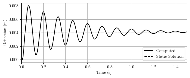
As shown in the computed results, the flexible wall undergoes damped, forced vibration and reaches the expected solution for deflection. Note, there is no structural damping in the model, only damping from the fluid mass.

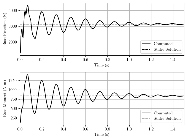
And for the reactions, there is some initial high frequency response, but the noise is damped out, and the computed solutions reach the statics-based solutions.

The next logical step is to impose a uniform excitation on a tank with flexible walls, but I’ll save that for another post.

OpenSees Cloud

OpenSees AMI

Hydrostatic Loading on a Wall