One Is All You Need

Original Post - 02 Mar 2025 - Michael H. Scott

Visit Structural Analysis Is Simple on Substack.

It is fairly well known that you can use a single force-based element to simulate the material nonlinear response of a frame member. Likewise, using a corotational mesh of displacement-based elements is an effective approach to simulate combined material and geometric nonlinearity.

A previous post looked at geometric nonlinearity with linear-elastic response in a single element. But using only one element per frame member to represent both material and geometric nonlinearity is a sort of holy grail for OpenSees analyses.

OpenSees has three frame element formulations that are capable of simulating material and geometric nonlinear response within the basic system:

dispBeamColumnNL – uses Green-Lagrange strain and accounts for moderate rotations in the element displacement field
forceBeamColumnCBDI – uses Lagrange polynomials to approximate the element displacement field from curvatures at the integration points
mixedBeamColumn – enforces strong equilibrium like the force-based formulation, but assumes a shape function for the element displacement field

When I first set out to write this post and compare these three element formulations, I picked what turned out to be a moderately difficult problem. So, I went back to (and modified) a standard test problem for geometric nonlinearity. The model is a simply-supported beam with an eccentric axial load applied at one end.

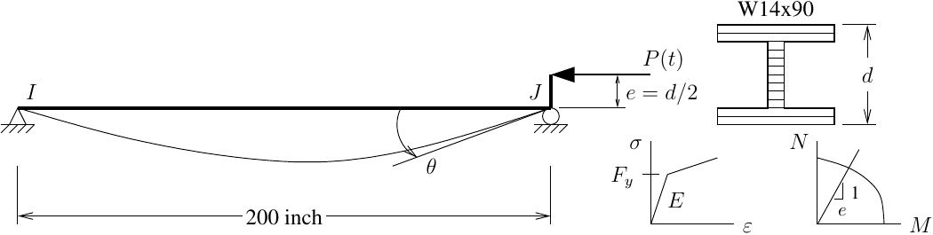
Simple beam with eccentric axial load

The beam is W14x90 with bilinear stress-strain response where E=29000 ksi and F_y=36 ksi with 5% strain-hardening ratio. Yeah, the strain-hardening is pretty high, but it let’s us crank in a lot of load and see the effects of combined material and geometric nonlinearity.

Five Gauss-Legendre points are used in each element formulation and each section is discretized into 6 web fibers and 4 fibers in each flange. The peak axial load is 0.8EI/L² with eccentricity equal to half the section depth.

import openseespy.opensees as ops

kip = 1
inch = 1
ksi = kip/inch**2

L = 200*inch
E = 29000*ksi
Fy = 36*ksi
alpha = 0.05
H = alpha/(1-alpha)*E

# W14x90
d = 14*inch
bf = 14.5*inch
tw = 0.44*inch
tf = 0.71*inch
I = 999*inch**4

# Load and eccentricity
Pmax = 0.8*E*I/L**2
e = 0.5*d

ops.wipe()
ops.model('basic','-ndm',2,'-ndf',3)

ops.node(1,0,0); ops.fix(1,1,1,0)
ops.node(2,L,0); ops.fix(2,0,1,0)

ops.uniaxialMaterial('Hardening',1,E,Fy,H,0)
ops.section('WFSection2d',1,1,d,tw,bf,tf,6,4)

ops.beamIntegration('Legendre',1,1,5)

ops.geomTransf('Linear',1)

ops.element('mixedBeamColumn',1,1,2,1,1,'-geomNonlinear')
# ops.element('forceBeamColumnCBDI',1,1,2,1,1)
# ops.element('dispBeamColumnNL',1,1,2,1,1)

ops.timeSeries('Linear',1,'-factor',Pmax)
ops.pattern('Plain',1,1)
ops.load(2,-1,0,e)

tmax = 1
Nsteps = 100
dt = tmax/Nsteps

ops.system('UmfPack')
ops.test('NormDispIncr',1e-8,10,0)
ops.integrator('LoadControl',dt)
ops.analysis('Static','-noWarnings')

for i in range(Nsteps):
    ops.analyze(1)

For each element formulation, the computed response is compared to the response obtained using one element of the formulation’s geometrically linear counterpart (dispBeamColumnNL to dispBeamColumn; forceBeamColumnCBDI to forceBeamColumn; and mixedBeamColumn with and without the -geomNonlinear option) as well as the exact solution. And by “exact solution” I mean the response obtained using a fine corotational mesh of displacement-based elements.

Note that the plastic axial load for this beam is 954 kip and the yield moment is 430 kip-ft. The beam yields at an applied axial load under 450 kip, with corresponding applied moment of about 260 kip-ft, indicating a high amount of axial-moment interaction.

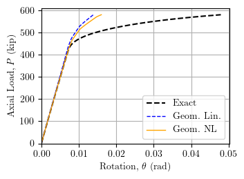
The computed axial load-rotation results are shown below for the displacement-based formulations. As expected, the single element solutions are stiffer and stronger post-yield compared to the exact solution.

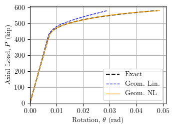
Response with displacement-based elements

The computed results for the force-based formulations are shown below. The geometrically nonlinear CBDI formulation is close to the exact solution.

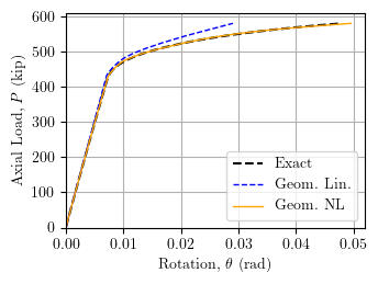
Response with force-based elements

Finally, the computed axial load-rotation results are shown below for hte mixed formulations. The geometrically nonlinear formulation agrees with the exact solution.

Response with mixed elements

While you can capture some geometric nonlinearity with a single dispBeamColumnNL element, you are better off to use either the forceBeamColumnCBDI or mixedBeamColumn (with -geomNonlinear option) if you would like to simulate combined material and geometric nonlinear with a single frame element.

OpenSees Cloud

OpenSees AMI

One Is All You Need