OpenSees Cloud

OpenSees AMI

OpenSees Coming and Going

Original Post - 10 Mar 2025 - Michael H. Scott

Visit Structural Analysis Is Simple on Substack.

Years ago, one of those shows like Diners, Drive-Ins, and Dives featured a greasy spoon somewhere in middle America famous for its eggs and fried chicken meal known as the “Coming and Going”–the boundary conditions of a chicken’s life on a single plate.

This quarter in Eastchester, I am teaching the introductory undergraduate course in structural analysis and the graduate level course in nonlinear structural analysis. Although no one will end up on a trucker’s lunch plate, I am in contact with students coming into structural analysis as well as those going out into the great structural analysis abyss.

Most of this blog deals with the abyss, showing something about nonlinear structural analysis with OpenSees. Only a handful of posts deal with fundamental structural analysis principles that juniors in civil engineering would recognize.

Sure, equilibrium, compatibility, and constitution run throughout all structural analysis courses. For example, in the nonlinear analysis course, it’s a lot of “here’s some algorithms and formulations and here’s how to do it in OpenSees, now let’s check that equilibrium is satisfied”. In the undergraduate course it’s “here’s some fundamental principles and here’s some output from OpenSees, now let’s interpret the output”. That I present analysis results obtained from OpenSees is not important for the undergraduate course–any structural analysis software would suffice.

But the students coming and the students going, they all see OpenSees.

While we can use OpenSees for the analysis of anything from static loading of statically determinate models to material and geometric nonlinear dynamic response histories, what can we do with influence lines? Essentially a side step between coming and going, influence lines are some kind of survivorship bias for me–never really learned them but I turned out OK.

Any way, the scripting capabilities of OpenSees make quantitative influence lines doable, although a bit arduous. But what about the Müller-Breslau principle for qualitative influence lines? Can we use OpenSees to demonstrate this juxtaposition of equilibrium and compatibility?

The Müller-Breslau principle says that to construct an influence line for X in a structural model, we should remove the ability of the model to resist X, then apply a unit load at and in the direction of X. The model’s resulting deflected shape is then proportional to the influence line for X.

For example, consider the two-span continuous beam shown below.

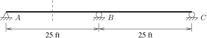
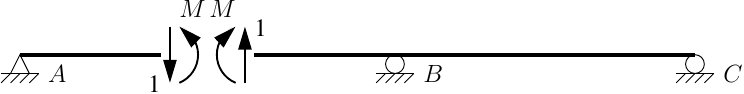
To construct an influence line for the internal bending moment at the middle of span AB, we insert a moment release then apply a unit internal moment at that location. The moment release transmits non-zero shear, V.

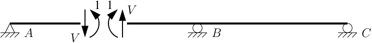
Likewise, we would insert a shear release and apply a unit internal shear in order to obtain the influence line for internal shear at midspan. The shear release transmits non-zero moment, M.

The OpenSees code for applying the Müller-Breslau principle is straightforward. The moment release is attained with two nodes and an equalDOF constraint between the translational DOFs with equal and opposite unit moments are applied on the two nodes. Similarly, the shear release is obtained with constraints on the horizontal and rotational DOFs along with equal and opposite unit transverse loads.

import openseespy.opensees as ops

kip = 1
ft = 1
inch = ft/12.0

L = 25*ft

# These values are not terribly important
A = 20*inch**2
I = 800*inch**4
E = 29000*kip/inch**2

ops.wipe()
ops.model('basic','-ndm',2,'-ndf',3)

ops.node(1,0,0); ops.fix(1,1,1,0)
ops.node(2,L/2,0)
ops.node(3,L/2,0)
ops.equalDOF(2,3,1,2) # Moment release
#ops.equalDOF(2,3,1,3) # Shear release
ops.node(4,L,0); ops.fix(4,0,1,0)
ops.node(5,2*L,0); ops.fix(5,0,1,0)

ops.geomTransf('Linear',1)

ops.element('elasticBeamColumn',1,1,2,A,E,I,1)
ops.element('elasticBeamColumn',2,3,4,A,E,I,1)
ops.element('elasticBeamColumn',3,4,5,A,E,I,1)

ops.timeSeries('Constant',1)
ops.pattern('Plain',1,1)
ops.load(2,0,0,1) # Unit moments
ops.load(3,0,0,-1)
#ops.load(2,0,-1,0) # Unit shears
#ops.load(3,0,1,0)

ops.analysis('Static','-noWarnings')
ops.analyze(1)

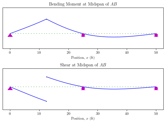
The deflected shapes, plotted below with opsvis, are proportional to the influence lines for the quantity of interest.

This post was a little scrambled, but it done came and went.