OpenSees Cloud
OpenSees AMI
Empty Spaces
13 Jan 2026 - Michael H. Scott
Recently, a large OpenSees model was posted in an online forum with the
poster asking why the analysis took longer than expected. Short answer:
Not only did using a heavy-duty recorder that writes all node, element,
and section data take up a big chunk of time, but using OpenSees’s
default linear equation solver, ProfileSPD, also incurred a
significant performance hit.
The model, generated with Alpaca4D, a Grasshopper plugin with OpenSees as its analysis engine, has just over 23,500 nodes and is a space frame lattice structure with about 140,000 equations.
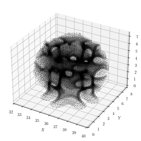
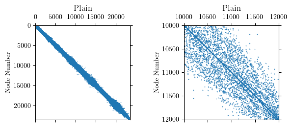
If you plot the model’s nodal connectivity, which is a proxy for the topology of the stiffness matrix, the system appears fairly banded. The connectivity matrix has 224,656 non-zeros and within the band, the entries are moderately dense.
Internally, OpenSees uses the reverse Cuthill-McKee algorithm (RCM) to
permute the node order for assigning equation numbers. The goal of RCM
is to reduce the bandwidth of the nodal connectivity matrix. Approximate
minimum degree (AMD), whose objective is to minimize fill-in during
factorization, is also available in OpenSees. For this model, RCM
produces a clearly defined, banded connectivity pattern.
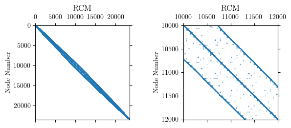
The RCM numberer did its job and reduced the bandwidth of the nodal
connectivity matrix to under 1000 nodes for this model. But the permuted
node order reveals significant sparsity in the system of equations.
What shall we use to fill the empty spaces?
With the ProfileSPD linear solver (the default in OpenSees), memory is
allocated in each column for all entries between the diagonal and the
furthest non-zero. This storage scheme is sometimes referred to as
“skyline” as the resulting pattern looks like a cityscape.
Likewise, for the BandSPD linear solver, memory is allocated within
the entire bandwidth. For this model, where the profile is essentially
the band, there is not much difference between ProfileSPD and
BandSPD in terms of memory and storage requirements.
With sparse matrix storage, used by the SparseSPD and other solvers in
OpenSees, only the non-zero entries are stored. In other words, we do
not fill the empty spaces. In addition, the solver only operates on the
non-zeros instead of chugging through zeros in the skyline or band.
For the lattice structure, using the SparseSPD solver on my modest
laptop, one analysis time step took 28.4 sec. This runtime is a bit high
for a variety of reasons that have nothing to do with the linear
equation solver. For example, the model uses forceBeamColumn elements,
each with five elastic sections, a choice that can make residual
evaluations more expensive than the matrix factorization itself.
Nonetheless, on this same machine, the ProfileSPD and BandSPD failed
to analyze within a reasonable amount of time. This outcome is
consistent with the sparsity of the system and the ensuing memory
requirements for profile and banded storage.
The default analysis options in OpenSees can kill performance on large, sparse models. Even moderately sized models with several hundred nodes and a few thousand equations will run much faster with a sparse equation solver.
