Minimal DDM Verification Example

05 May 2026 - Michael H. Scott

The direct differentiation method (DDM) computes the gradient, or sensitivity, of a structural response quantity with respect to model parameters. The DDM can be difficult to implement but produces accurate and computationally efficient derivatives of the structural response.

The standard approach to verify DDM implementations is by comparison with finite difference calculations where the response is re-computed with perturbed parameter values. However, there are cases where verification against closed form derivatives is possible.

Consider a linear-elastic cantilever with a point load at its free end.

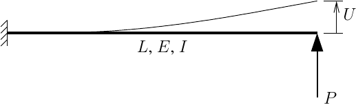
Cantilever of length L with point load P applied at its free end

The deflection at the free end, U=PL³/(3EI), depends on four variables. Closed-form derivatives define the exact sensitivity that the DDM should reproduce.

Elastic modulus, E
dU/dE = -PL³/(3E²I)
Second moment of area, I
dU/dI = -PL³/(3EI²)
Load magnitude, P
dU/dP = L³/(3EI)
Cantilever length, L
dU/dL = PL²/(EI)

Note that the derivatives with respect to E and I are negative, i.e., an increase in these parameters will lead to a decrease in deflection magnitude. On the other hand, the derivatives with respect to P and L are positive and an increase in their values will lead to an increase in deflection magnitude.

The algebraic signs confirm intuition, but the DDM-based gradients should match the analytical derivatives.

We can use these expressions to verify the OpenSees implementation of DDM-based sensitivity for a force-based frame element with elastic sections–essentially a unit test for maintaining correctness of the force-based element sensitivity implementation.

DDM-based sensitivity calculations can be added to an OpenSees script in three steps:

Define parameters for each variable of interest using the parameter command. This part can be non-intuitive as the strings passed to the parameter command depend on where the parameter resides within the OpenSees domain. Here, E and I are section properties, which are part of the element. The applied load is part of a load pattern and parametrizing the X-coordinate of node 2 effectively changes the element length without affecting the element formulation.
Declare a sensitivity algorithm, which is largely procedural and the best option is -computeAtEachStep in most cases.
After (or during) an analysis, use the sensNodeDisp command to retrieve the computed sensitivity with respect to each parameter.

import openseespy.opensees as ops
from numpy import isclose

E = 29000
A = 20
I = 800
L = 48
P = 5

ops.wipe()
ops.model('basic','-ndm',2,'-ndf',3)

ops.node(1,0,0); ops.fix(1,1,1,1)
ops.node(2,L,0)

ops.section('Elastic',1,E,A,I)
ops.beamIntegration('Legendre',1,1,2)

ops.geomTransf('Linear',1)

ops.element('forceBeamColumn',1,1,2,1,1)

ops.timeSeries('Constant',1)
ops.pattern('Plain',1,1)
ops.load(2,0,P,0)

# 1. Define parameters for E,I,P,L
ops.parameter(1,'element',1,'E')
ops.parameter(2,'element',1,'I')
ops.parameter(3,'loadPattern',1,'loadAtNode',2,2)
ops.parameter(4,'node',2,'coord',1)

ops.analysis('Static','-noWarnings')

# 2. Declare sensitivity algorithm
ops.sensitivityAlgorithm('-computeAtEachStep')

ops.analyze(1)

# 3. Compare sensNodeDisp to closed form solutions
# (node tag, dof, param tag)
assert isclose(ops.sensNodeDisp(2,2,1),-P*L**3/(3*E*E*I))
assert isclose(ops.sensNodeDisp(2,2,2),-P*L**3/(3*E*I*I))
assert isclose(ops.sensNodeDisp(2,2,3),L**3/(3*E*I))
assert isclose(ops.sensNodeDisp(2,2,4),P*L*L/(E*I))

The assertions pass and give a baseline for DDM verifications with material and geometric nonlinear response. If the assertions fail, we know there is an issue in the DDM-based modules of the element state determination.

OpenSees Cloud

OpenSees AMI

Minimal DDM Verification Example