OpenSees Cloud
OpenSees AMI
Break Your Concentration
17 Aug 2026 - Michael H. Scott
There are many reasons I’ve never been a huge fan of how concentrated plasticity models are typically implemented in OpenSees.
First, these models lump all material nonlinearity into a single point of zero length at each end of an elastic frame element. As a result, calibration is necessary to get from physically meaningful section response (moment-curvature, axial-moment interaction, etc.) to member-level response, e.g., moment-rotation.
Second, concentrated plasticity models double count the elasticity of the elastic frame element and the zero length springs. The typical workaround is to define the springs with very high initial stiffness, but issues with dynamic analysis ensue: high Rayleigh damping forces and potential residual flip-flop due to stiff unloading.
Finally, concentrated plasticity elements are difficult to define with two nodes at each end of the frame element, zero length elements, and equal DOF constraints to prevent rigid body motion. Inclined members with concentrated plasticity can get messy because the member axes do not coincide with the global axes in which the equal DOF constraints are defined.
Compared to distributed plasticity elements, especially those coupled with fiber sections, concentrated plasticity elements are touted to be the computationally efficient choice. But, given the extra nodes and constraints, issues with dynamic analysis, and necessary calibration, I’m not so sure that assumption is justified. Someone should compare the computational cost of the two approaches. Maybe me, just not today.
With my rant about how concentrated plasticity elements are implemented in OpenSees out of the way, let’s now focus on the objective of this post.
An example shown in Figure 10.5 from Jeffers’s textbook, Linear and Nonlinear Methods of Matrix Structural Analysis, uses stress resultant plasticity to couple the axial force and bending moment at concentrated plastic hinge locations.
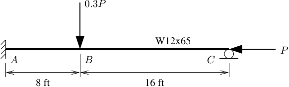
The member is a steel W12x65 shape (E=29000 ksi, Fy=50 ksi) with section properties A=19.1 inch2, Z=96.8 inch3, and I=533 inch4.
The yield surface is defined by the function n2+m2+3.5n2m2=1, where n=N/Np and m=M/Mp are the axial force and bending moment normalized by the plastic capacities Np and Mp, respectively. The post-yield response is elastic-perfectly-plastic (EPP).
Due to the axial-moment interaction, this example is a few steps beyond the typical OpenSees concentrated plasticity use case where only flexural springs are used. However, the example is not out of reach for OpenSees. I will replicate the analysis using material nonlinear force-based elements with a specialized beam integration. I could use zero length section elements, but I don’t want to condone that behavior.
Unfortunately, the yield surface used in the Jeffers example has not been implemented in OpenSees. Instead, we can use the Elliptical section model with yield surface n2+m2=1, then investigate the differences in response.
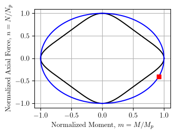
The inputs for the Elliptical section model are the section stiffnesses, EA and EI, the plastic capacities, Np=FyA and Mp=FyZ, and zero kinematic hardening and very small isotropic hardening ratio (α=1e-8). We can’t do all zeros for the hardening parameters because the analysis will fail to converge after a mechanism forms.
For the force-based elements, we will use the ConcentratedPlasticity beam integration. The advantage of this beam integration is we can use section force-deformation models directly in a frame element without all the gymnastics that accompany concentrated plasticity with zero length elements.
import openseespy.opensees as ops

kip = 1
inch = 1

ft = 12*inch
ksi = kip/inch**2

# W12x65
A = 19.1*inch**2
I = 533*inch**4
Z = 96.8*inch**3

E = 29000*ksi
Fy = 50*ksi

Np = Fy*A
Mp = Fy*Z

ops.wipe()
ops.model('basic','-ndm',2,'-ndf',3)

ops.node(1,0,0); ops.fix(1,1,1,1)
ops.node(2,8*ft,0)
ops.node(3,24*ft,0); ops.fix(3,0,1,0)

ops.section('Elastic',1,E,A,I)
ops.section('Elliptical',2,E*A,E*I,Np,Mp,1e-8,0,0,'P','Mz')

secTagE = 1
secTagI = secTagJ = 2
ops.beamIntegration('ConcentratedPlasticity',1,secTagI,secTagJ,secTagE)

ops.geomTransf('Linear',1)

ops.element('forceBeamColumn',1,1,2,1,1)
ops.element('forceBeamColumn',2,2,3,1,1)

ops.timeSeries('Linear',1)
ops.pattern('Plain',1,1)
ops.load(2,0,-0.3,0)
ops.load(3,-1,0,0)

Umax = 2*inch
Nsteps = 100
dU = Umax/Nsteps

ops.integrator('DisplacementControl',2,2,-dU)
ops.analysis('Static','-noWarnings')

ops.analyze(Nsteps)
Alternatively, we can use the HingeRadau beam integration with lpI=lpJ=1, but the ConcentratedPlasticity integration is easier.
In the textbook analysis, Jeffers reports the first plastic hinge at P=260 kip and the second plastic hinge at P=331 kip.
For the OpenSees analysis, the hinges form at P=288 kip and P=385 kip, which are higher loads than the textbook example because, for a given axial force, the elliptical yield surface permits larger bending moments than the yield surface used in the textbook example.
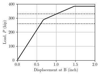
Although there is a lot more to investigate, this example showed that OpenSees can model concentrated plasticity using force-based frame elements and section stress resultant plasticity models, without the extra nodes, equal DOF constraints, calibration, and double-counted elasticity of the usual zero length element approach.