OpenSees Cloud
OpenSees AMI
A Minimal OpenSees Model Viewer
09 Sep 2026 - Michael H. Scott
Although there are several OpenSees post-processors out in the wild, creating your own model viewer for quickly checking a model definition and the analysis results is incredibly straightforward.
All you need is
matplotlib,
awareness of a few OpenSees utility functions, and a couple dozen lines
of Python code.
For example, to plot a 3D model of two-noded elements (frame, truss, link, etc.), you can use Python code built on these four OpenSees utility functions:
-
ops.getNodeTags– returns a list of all node tags currently defined in your model -
ops.nodeCoord– returns a list of the coordinates for a given node -
ops.getEleTags– returns a list of all element tags currently defined in your model -
ops.eleNodes– returns a list of node tags connected by a given element
The plot_model function plots to ax, a matplotlib Axes object.
import openseespy.opensees as ops
import matplotlib.pyplot as plt

def plot_model(ax):

    # Nodes
    for nd in ops.getNodeTags():
        XYZ = ops.nodeCoord(nd) # coordinates
        ax.plot(*XYZ,'ks') # black squares

    # Elements
    for ele in ops.getEleTags():
        nds = ops.eleNodes(ele) # connected nodes
        if len(nds) == 2:
            XYZ = ops.nodeCoord(nds[0]) + ops.nodeCoord(nds[1])
            ax.plot(XYZ[::3],XYZ[1::3],XYZ[2::3],'-k') # solid black lines
        else:
            #
            # Handle other element types
            #
            pass

ops.wipe()
ops.model('basic','-ndm',3,'-ndf',6)

#
# Define your model here
#

fig = plt.figure()
ax = fig.add_subplot(projection='3d')

plot_model(ax)

plt.show()
For an OpenSees model of the water tower described in
Björnsson and Krishnan (2014),
the plot_model function produces the following poorly-scaled, but
still useful, rendering:
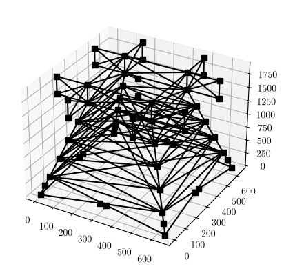
The distorted view is not because of the model itself, but rather the
bare bones plotting approach. To get consistent scaling, you can use the
ops.nodeBounds utility function and some matplotlib Axes functions
in your plot_model function.
# Physical bounds of the OpenSees model
xmin,ymin,zmin,xmax,ymax,zmax = ops.nodeBounds()

# Model center point
xc = 0.5 * (xmin+xmax)
yc = 0.5 * (ymin+ymax)
zc = 0.5 * (zmin+zmax)

# Common half-range
r = 0.5 * max(xmax-xmin, ymax-ymin, zmax-zmin)
# and some cushion
r *= 1.05

# Set axis limits
ax.set_xlim(xc-r, xc+r)
ax.set_ylim(yc-r, yc+r)
ax.set_zlim(zc-r, zc+r)
# and equal aspect ratios
ax.set_box_aspect([1, 1, 1])
Add this code either before or after the nodes and elements are drawn–it doesn’t matter.
Now the plot_model function gives a more realistic rendering of the
water tower model.
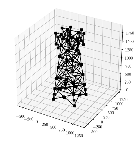
From here, you can play with colors, marker sizes, and line widths. You
can also add axis labels and node and element labels. Displaced shapes
and eigenmodes are straightforward using ops.nodeDisp and
ops.nodeEigenvector along with a magnification factor.
Another useful utility function is ops.eleType, which returns a string
that indicates the type of a given element. Knowing the element type is
important when rendering isonodal elements, e.g., a four-node shell
requires four lines while a four-node tetrahedron element requires six.
Built with only a few lines of code, the uncomplicated model viewer shown in this post is easily modified and extended to meet your needs.