OpenSees Cloud
OpenSees AMI
Heat Conduction in OpenSees
15 Oct 2026 - Michael H. Scott
I recently asked ChatGPT whether OpenSees can solve structural dynamics problems with no mass. Long story short, I ended up using OpenSees to solve one-dimensional heat conduction problems.
Using a structural dynamics solver to solve heat conduction problems is nothing new. In fact, heat conduction was the second assignment Prof. Taylor gave us in CE 233.
The governing equation for transient heat conduction is
\[{\bf C}_T\dot{\bf T}(t) + {\bf K}_T{\bf T}(t) = {\bf Q}(t)\]where T(t) is the nodal temperature vector, CT is the thermal capacity matrix, KT is the thermal conductivity matrix, and Q(t) is the heat input vector.
The governing structural dynamics equation is
\[{\bf M}\ddot{\bf U}(t) + {\bf C}\dot{\bf U}(t) + {\bf K}{\bf U}(t) = {\bf P}(t)\]So, we can use OpenSees’s structural dynamics architecture to solve heat conduction problems by:
- Interpreting nodal displacements as temperatures
- Representing thermal conductivity as structural stiffness
- Representing thermal capacity as structural damping
- Using zero structural mass
- Applying heat sources as nodal loads
- Imposing temperatures at boundaries via prescribed displacements
The above mathematical analogy is best shown by a simple example with a known solution.
A steel rod of length 0.1 m and cross-section area 0.01 m2, initially at 20° C throughout, is heated at its left end to 100° C and maintained while its right end is insulated. The thermal conductivity of the rod is k=45 W/(m-K), the specific heat is cp=470 J/(kg-K), and the density is ρ=7850 kg/m3.
An OpenSees model uses truss elements for heat conduction and zero-length elements with viscous materials for lumped thermal capacity. The thermal capacity matrix is analogous to structural mass, but in this model this matrix must operate on the structural “velocities” instead of accelerations. Alternatively, we could make a new FE_Element class that assembles thermal capacity contributions into damping forces, but let’s not get ahead of ourselves.
Also note that because nodal displacements correspond to temperature, we
can set the initial temperature along the rod using setNodeDisp() with
the -commit option. And prescribing the heated temperature at the left
end introduces a non-homogeneous single-point constraint, so we use the
Transformation constraint handler.
import openseespy.opensees as ops

k = 45 # Thermal conductivity, W/(m-K)
cp = 470 # Specific heat, J/(kg-K)
rho = 7850 # Density, kg/m^3

L = 0.1 # Length of rod, m
A = 0.01 # Cross-section area, m^2

Nele = 10 # Number of elements
dL = L/Nele

C = rho*cp*A*dL # Thermal capacity

To = 20 # Initial temperature, deg C
Th = 100 # Heated temperature, deg C

ops.wipe()
ops.model('basic','-ndm',1,'-ndf',1)

# Thermal conductivity
ops.uniaxialMaterial('Elastic',1,k)

# Truss elements for heat conduction
ops.node(0,0)
for i in range(1,Nele+1):
    ops.node(i,i*dL)
    ops.element('truss',i,i-1,i,A,1)

# Thermal capacity
ops.uniaxialMaterial('Elastic',2,0,C) # Viscous damping
ops.uniaxialMaterial('Elastic',3,0,C/2)

# Dashpots for lumped thermal capacity
for i in range(1,Nele+1):
    ops.node(-i,i*dL)
    ops.fix(-i,1)

for i in range(1,Nele):
    ops.element('zeroLength',-i,i,-i,'-mat',2,'-dir',1)
ops.element('zeroLength',-Nele,Nele,-Nele,'-mat',3,'-dir',1)

# Set initial temperature across rod
for i in range(0,Nele+1):
    ops.setNodeDisp(i,1,To,'-commit')

# Set heated temperature at left end
ops.timeSeries('Constant',1)
ops.pattern('Plain',1,1)
ops.sp(0,1,Th)

ops.integrator('Newmark',0.5,0.25)
ops.constraints('Transformation')
ops.analysis('Transient','-noWarnings')

tfinal = 600 # 10 minutes
dt = 1
Nsteps = int(tfinal/dt)

for i in range(Nsteps):
    ok = ops.analyze(1,dt)
    if ok < 0:
        break
The evolution of temperature at the ends and the center of the rod is shown below. As expected, the temperature along the rod approaches the prescribed temperature imposed at the heated left end. In addition, the computed solution matches the closed-form solution to the governing differential equation.
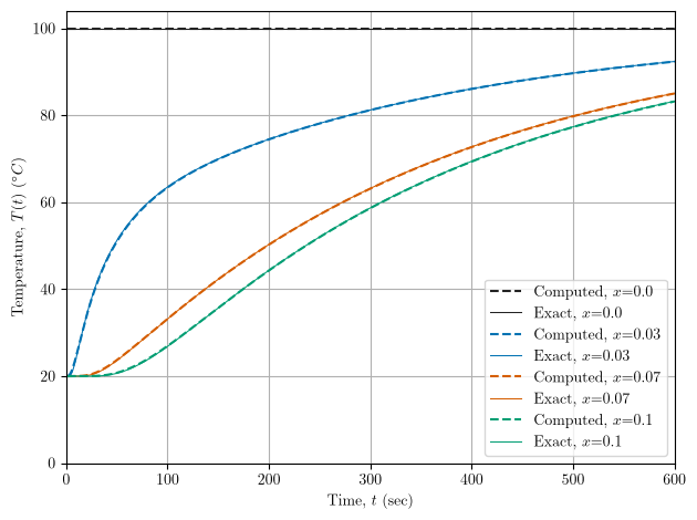
For this example, the constant (average) acceleration Newmark method (the default in OpenSees) gives stable results. Other time integrators could be used. For example, what happens if you use Newmark with linear acceleration for this problem? A broader discussion of numerical stability is beyond the scope of this post.