Static Analysis with Uniform Excitation

Original Post - 28 Jul 2024 - Michael H. Scott

The UniformExcitation defines reference nodal loads in proportion to the mass (nodal plus element contributions), multiplied by negative acceleration, which is specified in a time series. There’s nothing inherent in its implementation that ties the UniformExcitation to only dynamic analysis and earthquake excitations.

So, if I had known sooner that the UniformExcitation load pattern works in a static analysis, a few posts would have been much easier to write.

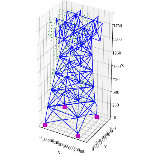
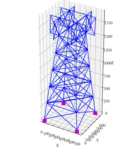
Rather than use simple 1D models to show what I mean, in this post I will use an OpenSees model of a water tower developed by Björnsson and Krishnan (2014), plotted below using opsvis.

Water tower model

This model has been used as a project for several on-campus and Ecampus deliveries of nonlinear structural analysis (CE 537) in Eastchester.

Gravity Loads

For frame models, it’s usually straightforward to define mass and weight separately at each node. There’s nothing wrong with that approach.

But let’s suppose you have defined the mass in your frame model and you don’t want to define gravity loads manually. The following code will impose gravity loads, without you having to define nodal loads.

#
# Define your model, include mass
#

DIR = 3 # 1 = X, 2 = Y, 3 = Z

ops.timeSeries('Constant',1)
ops.pattern('UniformExcitation',1,DIR,'-accel',1,'-factor',g)

ops.system('UmfPack')
ops.integrator('LoadControl',0.0)
ops.analysis('Static')
ops.analyze(1)
ops.reactions()

Note that the UniformExcitation will flip the sign on acceleration so that loads are applied in the negative Z-direction (or whatever direction you want). Thus, the positive g as the scale factor.

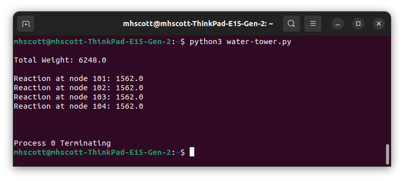
With the mass of the water tower model prescribed in Björnsson and Krishnan (2014), applying a uniform excitation gives a vertical reaction of 1562 kip at each support. The total weight of the water tower is 6248 kip.

Reactions at base of water tower

This approach to defining gravity loads will work for any frame or solid model, and will also work for element mass density (as long as the elements in your model implement getResistingForce() correctly, e.g., as shown here).

With the UniformExcitation, all the rigmarole with the Diagonal system, the GimmeMCK integrator, the printA function, and loops shown in this post is rendered unnecessary.

The Rayleigh Quotient

We can obtain an approximate mode shape for a model by applying static loads in proportion to the mode’s distribution of mass. This mode shape can then be used to calculate the Rayleigh quotient, which usually gives a very good approximation of the fundamental period.

A previous post showed the Rayleigh quotient for a 1D model, and in doing so, avoided a lot of complication with applying the mass-proportional loads. But now, the UniformExcitation makes the load application much easier for any size model.

#
# Define your model, include mass
#

DIR = 1 # 1=X, 2=Y, 3=Z
a = 0.01*g

ops.timeSeries('Constant',1)
ops.pattern('UniformExcitation',1,DIR,'-accel',1,'-factor',-a)

ops.analysis('Static','-noWarnings')
ops.analyze(1)

num = 0; den = 0
for nd in ops.getNodeTags():
    for dof in range(1,DOF+1):
        mj = ops.nodeMass(nd,dof)
        uj = ops.nodeDisp(nd,dof)
        num += mj*uj
        den += mj*uj*uj
    
# Rayleigh quotient
w2 = a*num/den
# Eigenvalue
w2 = ops.eigen(2)[0]

Again, note that the UniformExcitation will flip the sign on the acceleration, thus the negative acceleration. Here, a small acceleration (0.01*g) is used so that model response is not nonlinear.

The code above assumes all nodal mass. You’re on your own calculating the Rayleigh quotient if you use elements with mass density. However, after doing a static analysis with UniformExcitation, you can use GimmeMCK and printA to get the assembled mass matrix, then do scalar triple products with the nodal displacements.

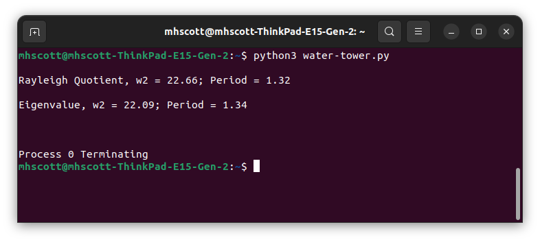
For vibration of the water tower model in the X-direction, the Rayleigh quotient gives 22.66 rad²/sec², which corresponds to a natural period of 1.32 sec. Eigenvalue analysis of the model gives 22.09 rad^{2</suo>/sec² and 1.34 sec.}

Natural period of water tower model

Load Control Pushover

Because the UniformExcitation defines a reference load pattern, we can use this pattern to perform a load-controlled pushover analysis.

In their paper, Björnsson and Krishnan (2014) did a pushover analysis of the water tower based on dynamic response to a “slow, ramped, horizontal ground acceleration that increases at a constant rate of 0.3g/min”. Talked about this approach to pushover analysis in this post, but didn’t really go into much detail.

But now, with the UniformExcitation, we can perform static analysis marching through pseudo-time with a linear time series and factor equal to the 0.3g/min jerk.

sec = 1
min = 60*sec

#
# Define model, include mass
#

DIR = 1 # 1=X, 2=Y, 3=Z

ops.timeSeries('Linear',1)
ops.pattern('UniformExcitation',1,DIR,'-accel',1,'-factor',-0.3*g/min)

Tfinal = 180*sec
dt = 1*sec
Nsteps = int(Tfinal/dt)

ops.integrator('LoadControl',dt)
ops.analysis('Static','-noWarnings')

ops.analyze(Nsteps)

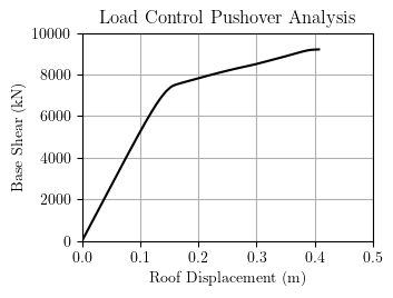
The base shear-roof displacement response of the water tower model is shown below. The analysis fails to converge at a base shear of about 9000 kN.

Load-displacement response using load control

The deformed shape of the water tower model (scale=10) at the final analysis step shows the first story braces beginning to buckle.

Displaced shape of model after load control

Because the UniformExcitation defines load in proportion to the mass distribution of the model, we essentially just did a first mode modal pushover.

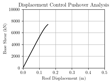
Displacement Control Pushover

Widely known and shown in the previous section, load-controlled pushover analyses are not able to track post-peak response, which may or may not be important (probably not important in this case). But if you do want the post-peak response, displacement control is the way to go.

Just like load control, the UniformExcitation defines a reference load pattern based on the distribution of mass, then we control the displacement at a single DOF. You don’t have to apply a reference load at and in the direction of the controlled DOF–node 700, referenced in the code below, is on the roof of the water tower model.

#
# Define model, include mass
#

DIR = 1 # 1=X, 2=Y, 3=Z

ops.timeSeries('Linear',3)
ops.pattern('UniformExcitation',2,DIR,'-accel',3,'-factor',-0.1*g)

Umax = 0.6*m
Nsteps = 200
dU = Umax/Nsteps

ops.integrator('DisplacementControl',700,DIR,dU)
ops.analysis('Static','-noWarnings')

ops.analyze(Nsteps)

Also, note that the 0.1*g factor applied in the UniformExcitation leads to large enough loads to make the water tower displace, but not so small or so large that the displacement controlled analysis has convergence issues.

The base shear-roof displacement response of the water tower model is shown below. The displacement-control solution is able to capture the post-peak response.

Load-displacement response using displacement control

The final deformed shape (scale=10) shows buckling of the braces in the first story of the water tower model.

Displaced shape of model after displacement control

That you can do so much with the UniformExcitation in OpenSees is another testament to Frank’s good software design.

OpenSees Cloud

OpenSees AMI

Static Analysis with Uniform Excitation

Gravity Loads

The Rayleigh Quotient

Load Control Pushover

Displacement Control Pushover