OpenSees Cloud
OpenSees AMI
Statically Equivalent Loads
14 Apr 2025 - Michael H. Scott
When it comes to numerical integration, OpenSees users either pay too much, or too little, attention.
Me? I pay way too much attention to the topic. How else did OpenSees end up with so many integration methods for frame elements?
But numerical integration is one of the concepts that users of OpenSees, or any other finite element analysis software, must understand.
Typical uses of numerical integration include beam fiber sections, layered shell sections, and element integrals where closed form solutions are not possible for arbitrary nonlinear material response. The trick is knowing when using more integration points will improve your results, or only increase your run-times.
While volume integrals for element resisting force and stiffness are the main applications of numerical integration, a recent question reminded me that we can also use numerical integration to develop statically equivalent loads.
The question was how to use OpenSees to analyze a simple beam with a quadratically increasing distributed load.
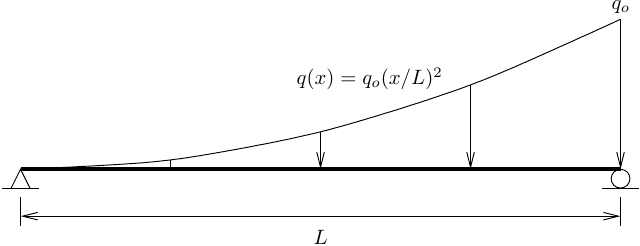
Quadratic member loads are not implemented in OpenSees because you don’t see this type of loading all that often out in the wild.
The beam is statically determinate, so we can show the vertical reactions are qoL/12 and qoL/4, and the exact solution for the internal bending moment is
\[{\displaystyle M(x)=\frac{q_oL^2}{12} \left( \left(\frac{x}{L}\right)^4 - \frac{x}{L} \right) }\]Assuming the beam is linear-elastic and prismatic, the exact solution for the transverse deflection is
\[{\displaystyle u(x)=\frac{q_oL^2}{12EI} \left( \frac{x^2}{30}\left( \frac{x}{L}\right)^4 - \frac{x^2}{6}\left( \frac{x}{L}\right) + \frac{2L}{15}x \right) }\]The standard modeling approach is to subdivide the beam into multiple elements of equal length, then use either nodal loads or member loads to approximate the quadratic loading function. Five or six elements will do the job.
But even with trapezoidal distributed loads applied over each subdivided element, you’ll never get the total load exactly right, i.e., you can’t get a perfect, statically equivalent loading. This error in approximating the load is usually not a big deal.
However, we can use quadrature to turn the analytical loading into a series of point loads. Because the loading function is quadratic, we can use as few as two Gauss points to make a statically equivalent loading.
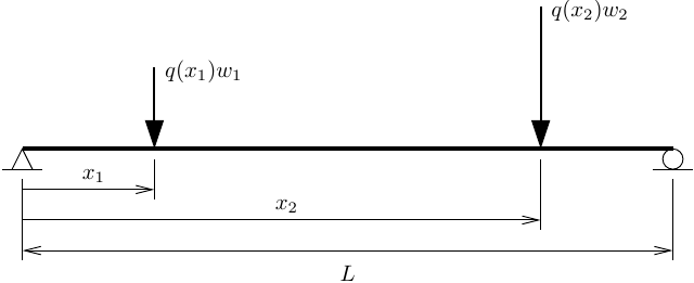
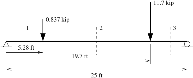
Using a single force-based element, we will need at least three Gauss points in the element to integrate the fifth order polynomials that result from the product of the fourth order curvature distribution with the linear weighting function.
For L=25 ft and qo=1.5 kip/ft, the loads and locations are shown below (to three significant figures).
And a simple OpenSeesPy model uses the
numpy.polynomial package
to define the statically equivalent loads as beamPoint member loads.
import openseespy.opensees as ops
from numpy import polynomial
from math import isclose

kip = 1
ft = 1

inch = ft/12
ksi = kip/inch**2

L = 25*ft
qo = 1.5*kip/ft

E = 29000*ksi
A = 20*inch**2
I = 800*inch**4

def q(x):
    return qo*(x/L)**2

Npbeam = 3
Npload = 2

ops.wipe()
ops.model('basic','-ndm',2,'-ndf',3)

ops.node(1,0,0); ops.fix(1,1,1,0)
ops.node(2,L,0); ops.fix(2,0,1,0)

ops.geomTransf('Linear',1)

ops.section('Elastic',1,E,A,I)
ops.beamIntegration('Legendre',1,1,Npbeam)

ops.element('forceBeamColumn',1,1,2,1,1)

pts,wts = polynomial.legendre.leggauss(Npload)
wts = L/2*wts
pts = L/2*(pts+1)

ops.timeSeries('Constant',1)
ops.pattern('Plain',1,1)

for i in range(Npload):
    x = pts[i]
    ops.eleLoad('-ele',1,'-type','beamPoint',-wts[i]*q(x),x/L)

ops.analysis('Static','-noWarnings')
ops.analyze(1)

ops.reactions()

assert isclose(qo*L/12,ops.nodeReaction(1,2))
assert isclose(qo*L/4, ops.nodeReaction(2,2))
The assertions on the vertical reactions confirm the applied loads are statically equivalent to the original quadratic loading.
With two Gauss points to represent the load and three Gauss points to represent the element response, the results are decent.
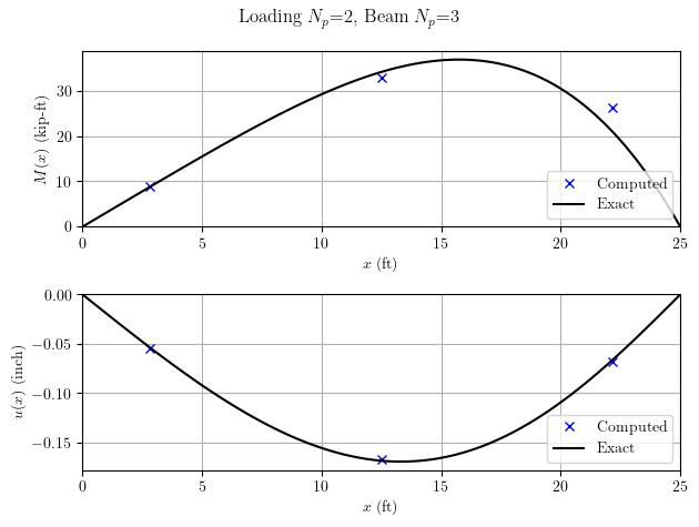
Although the total load is correct, the discretization of the loading
function into two point loads is too coarse to get good internal forces
and deflections. You can obtain the bending moment and transverse
deflection at each element integration point using the sectionForce
and sectionDisplacement commands.
Using six Gauss points for the loading while keeping three Gauss points for the element gives the following results, which look better for the internal bending moment.
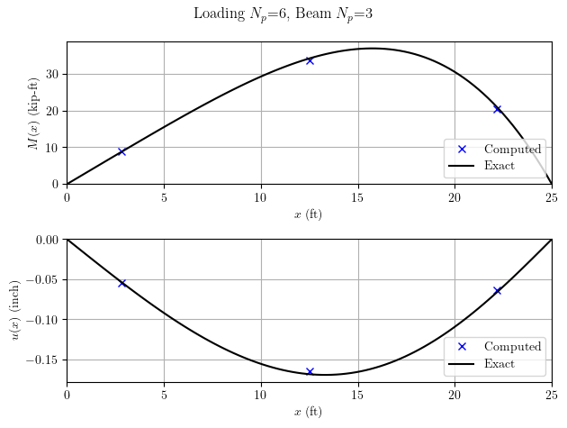
The load locations and magnitudes are shown below to three significant figures. I made a table because it’s too difficult to make a figure that’s not overly crowded.
| Load Number | Location (ft) | Magnitude (kip) |
|---|---|---|
| 1 | 0.844 | 0.00366 |
| 2 | 4.23 | 0.194 |
| 3 | 9.52 | 1.27 |
| 4 | 15.5 | 3.36 |
| 5 | 20.8 | 4.67 |
| 6 | 24.2 | 3.00 |
Play around with the number of integration points for the loading and the element response. This analysis takes some work, but it’s a different take on the standard approach of subdividing the member into multiple elements.